
Object Detection using Overfeat
This is part 1 of multi-part series on Object Detection. See Part 0.
A detailed tutorial is available in YouTube. The same topic is covered in brief in this blog.
ConvNet’s input size constraints
Problem - ConvNet’s input size constraints
The problem we discussed in the previous part was that, using the Sliding window technique and taking the crop of the image at different locations, I am ending up with too many inputs to my Localization network.
The reason why I have to take crops and resize them is that, the ConvNets expect fixed sized image inputs.
To solve this problem, let’s first understand why the ConvNets expect fixed size inputs. If we understand this, may be, we will be able to fix this.
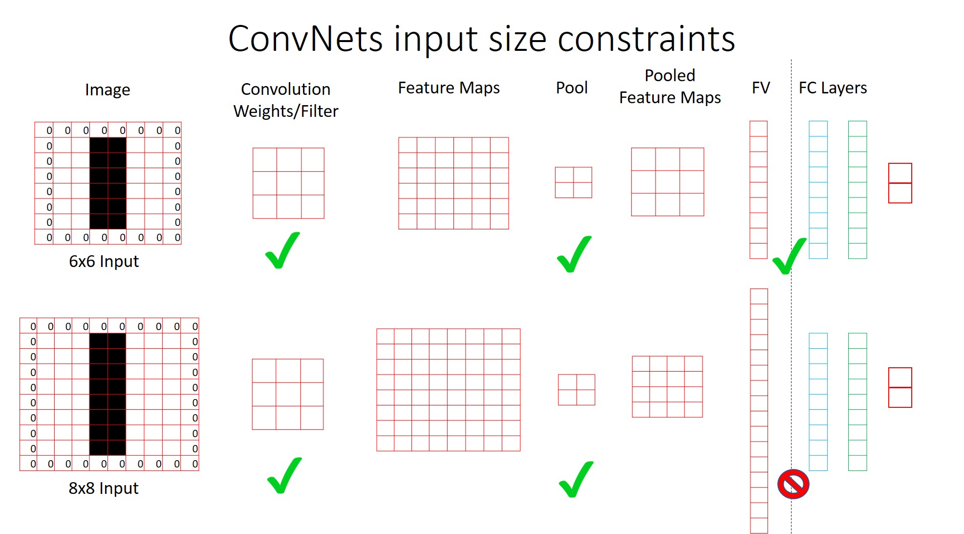
Briefly, the 3 main operations going on in the ConvNets are Convolution, Pooling and Fully Connected operations.
As you might be knowing, Convolution and pooling operations can be done on inputs of any size.
But the Fully Connected layer operations are done using ‘Dot Product’ of vectors.
And when you are taking dot products, the size of input and size of the filter should be the same. Else, the operation fails.
So, this is where the restriction is coming from.
Note: In this figure, assume each square is a pixel. You have ‘white’ pixels in 1st 2 columns, followed by ‘black’ and then ‘white’ pixels. The surrounding ‘zeros’ are for padding during convolution. The top row has a 6x6 image input and the 2nd row has 8x8 image input with the same Network.
See detailed discussion here
Solution - FC Layer implemented as Convolution operation.
Now that we have understood the root cause of the problem, how do we fix this?
One option available to us is that, we can implement the FC layer as a Convolution operation.
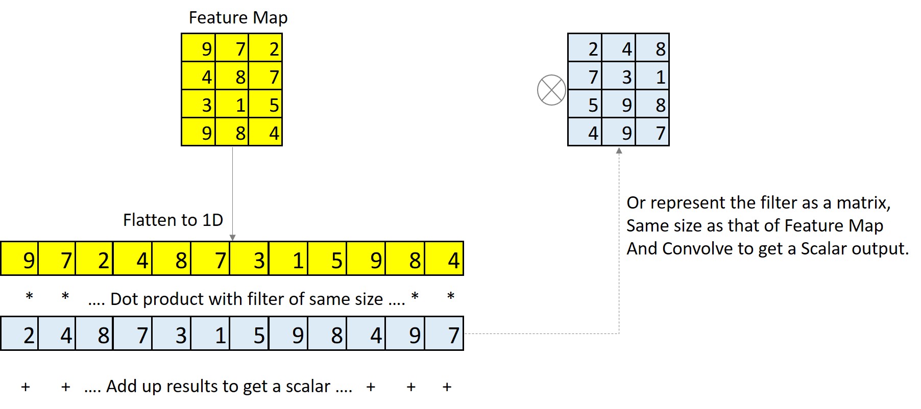
As you might be aware, usually, what is done is, the pooling layer output is flattened to a 1D vector. Then using a filter of same size, we take the dot product.
Instead, what you can do is, take the Pool layer output without flattening. This will be in the form of a mxn matrix. Take the same filter used for FC operation and represent it as a matrix of mxn dimension. Now, if you convolve the Pool layer output Feature Map with this filter matrix, you will get the same scalar output as that of the dot product.
See detailed discussion here
This way, we can implement the Fully Connected layer operation as a convolution operation.
Since convolution operations have no size constraint, this will remove the fixed size restriction.
Receptive Field & Spatial Output
Problem - I get more outputs than I need
But if you observe the output of this operation, you will see that, you will end up with different sized outputs.
For a 6x6 image with a 3x3 convolution with Stride=1 and Padding=1 and 2x2 Pooling, the output will be a 3x3 matrix.
With FC layer converted to Convolution operation, I have to use a 3x3 filter, which gives me a 1x1 output.
But if I scale this image (Image Pyramid) to 8x8, the output of the network will be 2x2. What I am expecting is just 1 output per class. But here I am getting 2 outputs per class. (Assuming there are 2 classes)
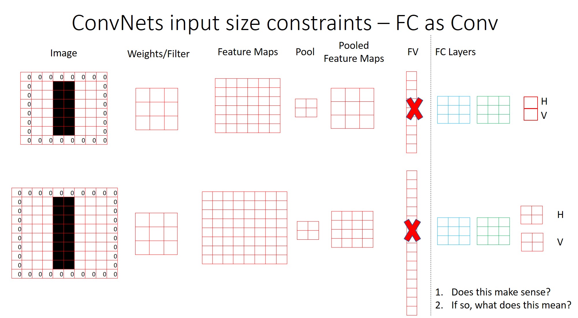
Now the question is, does this make sense? If so, what does this 2x2 output mean?
Receptive Field
Before we answer this question, we need to understand the concept of Receptive Field.
If we get a 1x1 output from a 4x4 patch of the image, we can say that, the receptive field of the network is 4x4. That is, each pixel in the output encodes information from a 4x4 patch of the image.
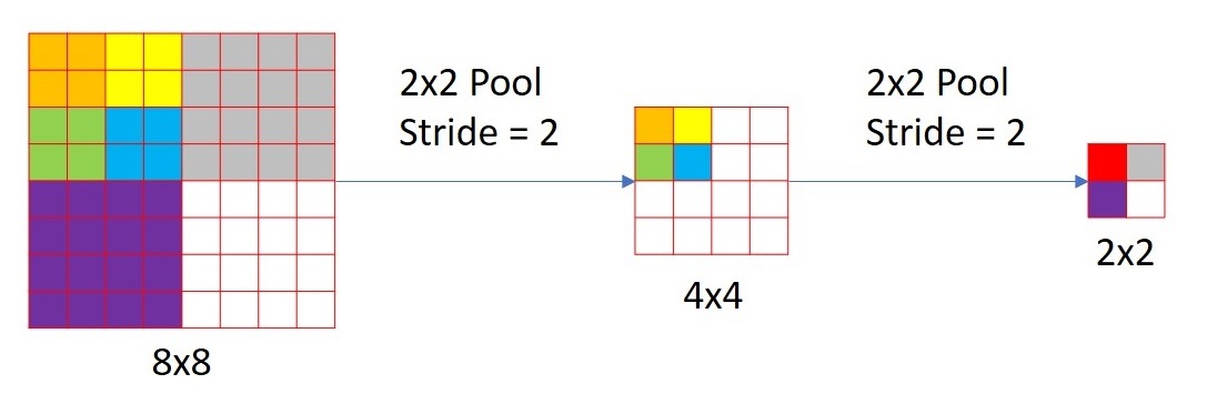
Similarly, if we run a 8x8 image through the same network, we get a 2x2 output.
In the figure below, for the 8x8 input, the ‘Red’, ‘Grey’, ‘Purple’ and ‘White’ pixels in the output encode the calculations on ‘Multi-coloured’, ‘Grey’, ‘Purple’ and ‘White’ patches of the image. Each of the patches are of size 4x4.
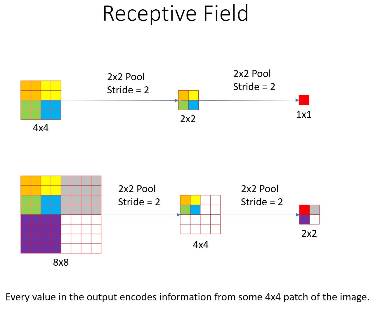
This 2x2 output is called as the Spatial Output.
No Problem - Its ‘Spatial Output’
Coming back to our original problem, we are getting a 2x2 output for the toy network of ours.
Here, the Receptive Field of the network is 6x6 as can be seen below.
With Spatial Outputs, we can detect different objects at different locations of the image. Below figure shows a 2x3 Spatial Output for a sample image.
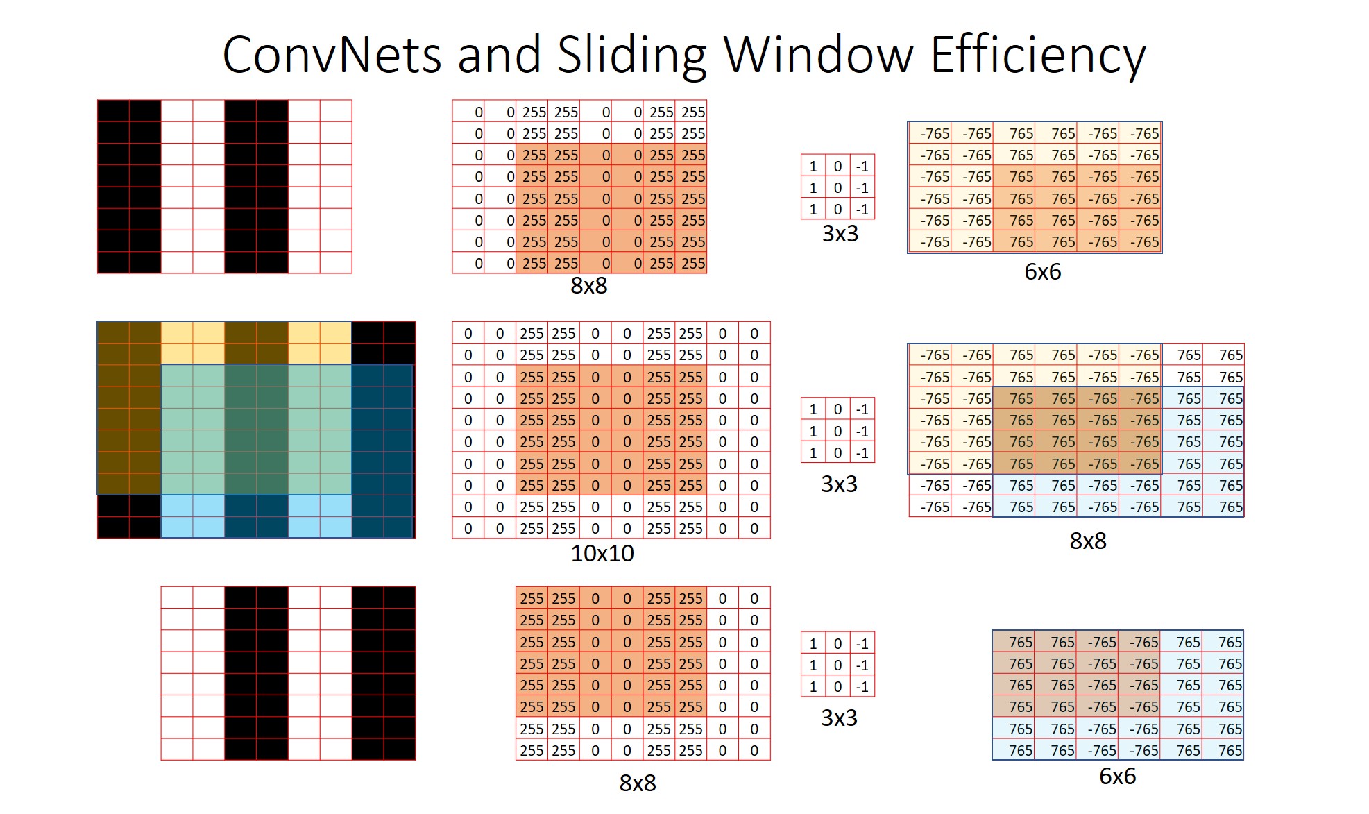
ConvNets Sliding Window Efficiency
Not only is the Convolution Operation in the FC layers convenient, it is also efficient, since we are using ‘Sliding Window’ technique.
This is because, using Sliding Window technique avoids repeated computations, which we would have incurred if we had taken the image crops.
Below figure shows a 10x10 image in the middle row. Lets say, we take 2 8x8 crops - top left and bottom right and do the convolutions separately. In the middle row, the convolution operation is applied to the entire image at once. We can see that, the outputs are necessarily the same. The top and bottom rows are just doing repeated computations in the overlap region (orange region) with no change in output.
Overfeat
Overfeat Intuition
By putting all the concepts we have learnt till now, we will be able to understand Overfeat. By converting the FC layers into convolution operation, we have removed the fixed input size constraint. There are 3 advantages to this:
- I can use the same localization network, without using the Sliding Window crops at different locations.
- Since there are no input size constraint, I will be able to use the Image pyramids.
- Since, I am using Image Pyramids, I will get the Spatial Output, which will give me detections at different locations of the image.
- Since the entire network is using Convolution operations, it is way more efficient than taking crops.
This the intuition behind OverFeat Network.
This Network won the ImageNet 2013 localization task (ILSVRC2013) and obtained very competitive results for the detection and classifications tasks.
See detailed discussion here
Overfeat Classification Network
This is the Overfeat Classification Network. It uses a modified AlexNet architecture for Convolution operations.
The first FC layer has 5x5 filter and 2nd and 3rd have 1x1 filters. The depth at both layers are 4096 each.
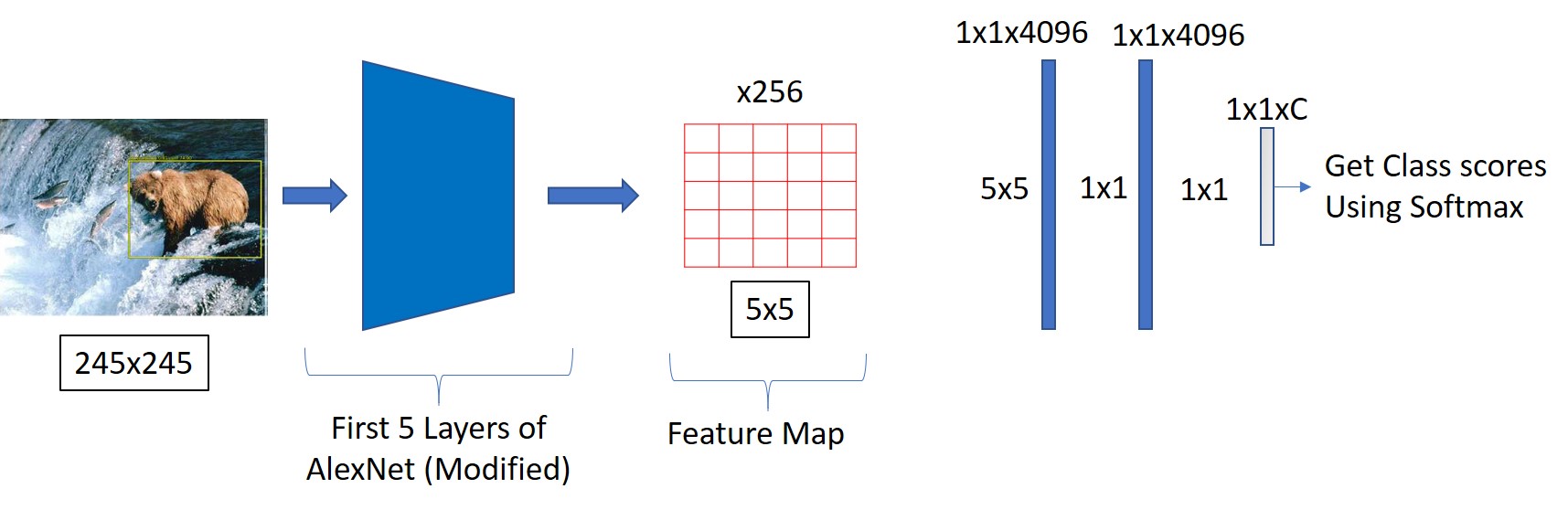
Let’s look at the FC layers in detail. Here, I have shown only the filter sizes without the depth.
But, how would you change the design to get a depth of 4096 at 2nd and 3rd FC layers?
As you know, to get M Feature Map outpus from N input Feature Maps, we need MxN filters.
In the below image for example, with 3 Feature Map inputs, we need 3 filters to get 1 Feature Map output. But, if we need 6 FM outpus, we need 6 such sets of filters. In total, we need 6x3=18 filters.
Detailed discussion on ConvNet Depth is here:
Similarly, to get a Feature Map output of depth 4096, at the 1st FC layer, we need 256*4096 filters. And each filter is of size 5x5. 256 - Since, the depth of AlexNet Conv layers is 256.
On the same lines, at the 2nd FC layer, we need to have 4096 filters, each of size 1x1.
The depth of the last FC layer, depends on the dataset. If we are using PascalVOC, it has 20 classes. We also need to account for the case, where the image patch contains no object or an unknown object. For this, we add one more class called ‘Background’.
So, in total we have 21 classes. To keep it generic, let us call this C.
Accordingly, the depth of last FC layer will be 4096*C and each filter will be of 1x1.
See detailed discussion here
Overfeat Detection Network
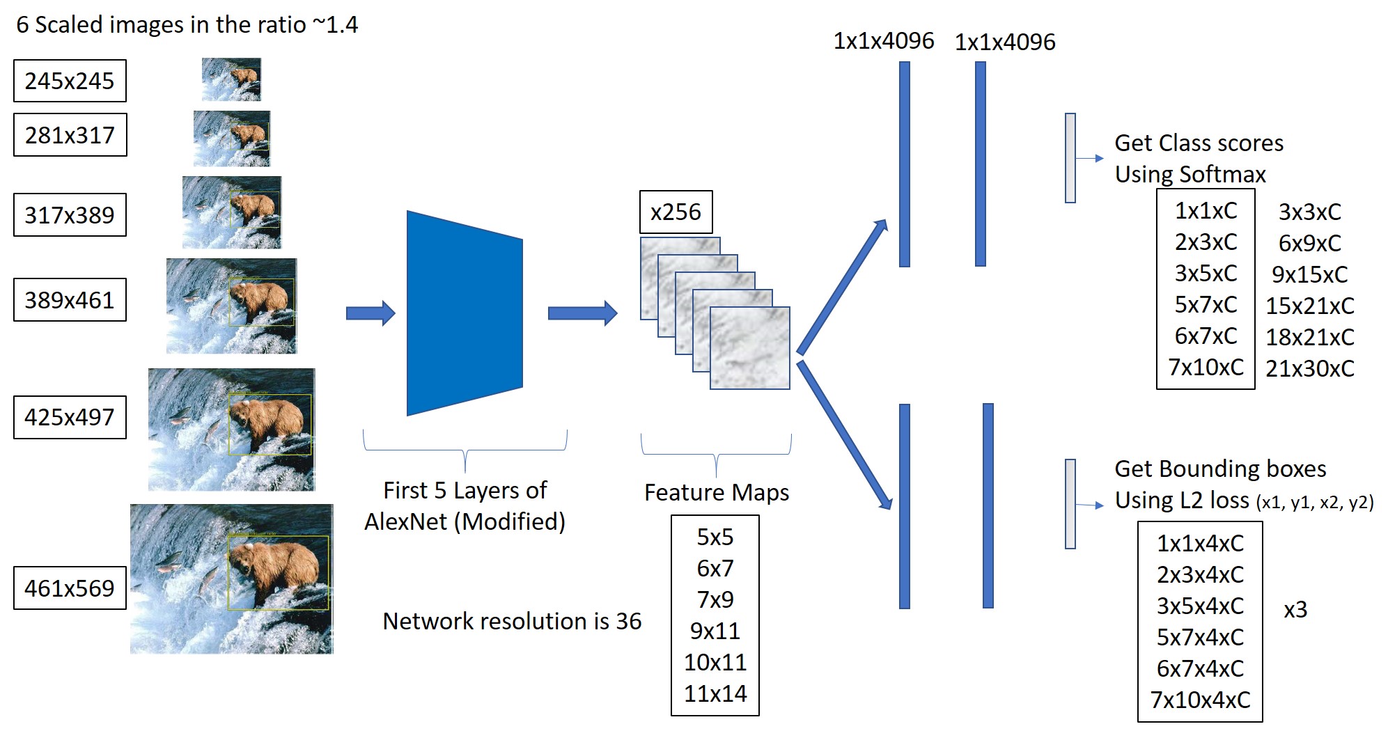
For Object Detection, Overfeat used an Image Pyramid of 6 different scales as shown below. Accordingly, the sizes of the Conv Feature Maps and the output Feature Maps change.
It is in the Detection Network, that we get the Spatial Output. Overfeat does not use Image Pyramids for Classification.
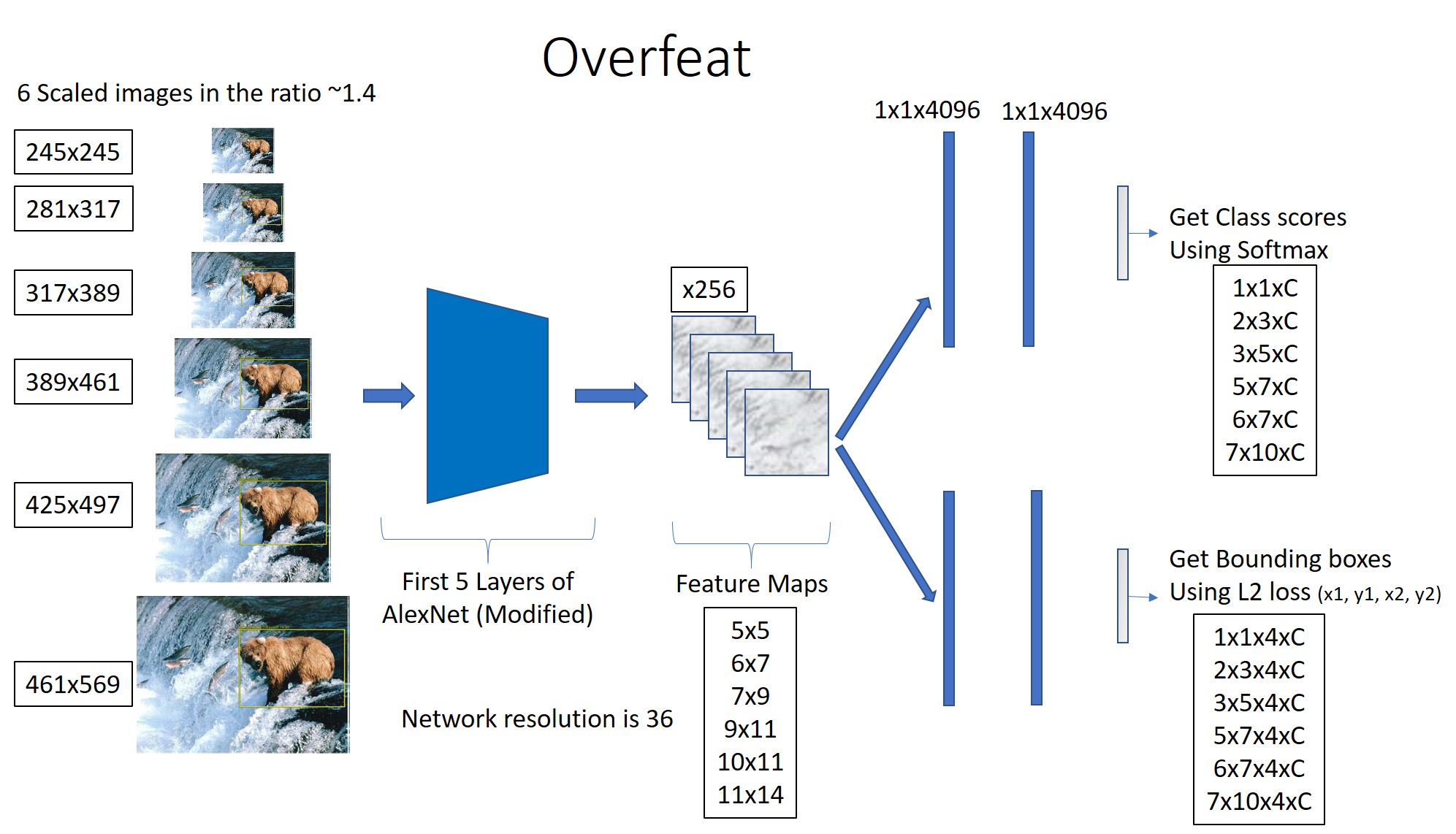
As an example, I am showing the Network for an Image Pyramid of size 281x317. (Ignore the values for 245x245, it is only for reference). For this image size, we get a 2x3 Spatial Output.
The Spatial Outputs for all other Image Sizes are shown below.
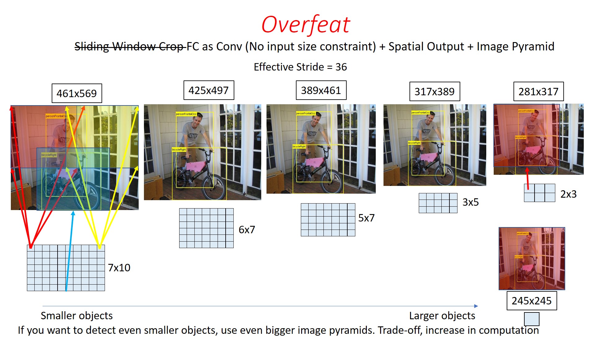
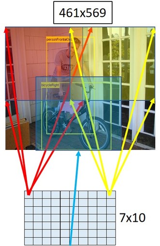
Here, we can see (not to scale), the Receptive field of different pixels of the Spatial Output for a 461x569 sized Image.
1x1 Convolution, Model Size, Effective Stride
1x1 Convolution and Model Size of ConvNet
See detailed discussion on calculating Model size of ConvNet here.
In the below image, we can see the size of FC layers when we use 1x1 Convolutions. It comes to around 45MB.
And, we get the same size, even if we use the dot product operations.
But, the advantage of 1x1 convolutions becomes significant when we take larger images.
Here, even for a 281x317 image, there is no increase in the model size for 1x1 Convolution case. But if FC layers are implemented as dot product operations, we get a significant increase in the model size (365MB).
So, that is how, the model size in Overfeat network remains constant irrespective of the size of the image that we use. This is the advantage of using 1x1 convolutions.
So, using 1x1 convolutions is one way of reducing the model sizes of your ConvNets, while not significantly compromising on the accuracy. This is something that can be kept in mind if you are designing any network.
Effective Stride of a Network
This is one more concept that you should be aware of.
Effective Stride basically tells you, by how many pixels you are shifting your focus at the input side if you move by 1 pixel in the Spatial Output.
Ideally your Effective Stride should be as low as possible, to ensure you are scanning all possible areas of the image.
For example, the effective stride of this network is 4.
For this network, effective stride is 2.
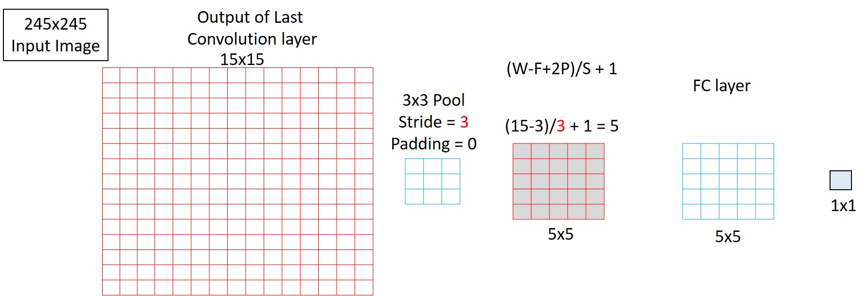
Effective Stride of Overfeat network is 36. But, if you want to improve this, that is, reduce the effective stride, you can employ a simple trick.
Below, you can see the input to the last Pooling layer in Overfeat. It is of size 15x15.
Overfeat uses a 3x3 pool with stride of 3 and 0 padding in the last pooling layer. With this, you get a 1x1 Spatial Output for a 245x245 image.
And to improve the Effective Stride, you can change just the stride to 2 from 3. With this you will be able to get a 3x3 output. And this is what is done in Overfeat for higher accuracies.
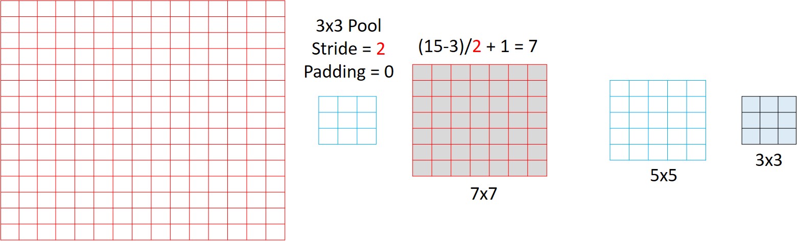
The modified Spatial Output sizes are shown below. Instead of 1x1xC, you will get a 3x3xC. Similarly for all other cases.
See detailed discussion here
Post processing at Output side
Confidence Score thresholding
Once we get the Spatial output, we will have multiple detections, each with different confidence scores. But the detections with low confidence scores will mostly be of background regions of the image and not that of any object. So we usually set a threshold of say 50% or 70% and eliminate all the bounding boxes that have lower scores than this.
Non Max Suppression
After Confidence thresholding, there is one last problem remaining. That is, there will be multiple detections per object.
For example, in the below figure for a 2x3 Spatial output, we get 2 detections for the left cat and 4 for the right one. For each cat, only one of these detections is valid or more accurate.
The question is, how do we select the best out of those multiple detections.
Option 1:
- Select the bounding box with the highest confidence score.
- And then remove all the boxes that overlap it.
This way, for the left cat, assuming that the red box has higher score than the yellow one, we eliminate the yellow one.
For the right cat, assuming that the green box has the highest score, we eliminate all the blue ones.
But this strategy may not work in all cases. Especially when the objects are close to each other. Consider the image below. The bounding boxes for both the persons overlap. (Left is Federer and right is Sachin)
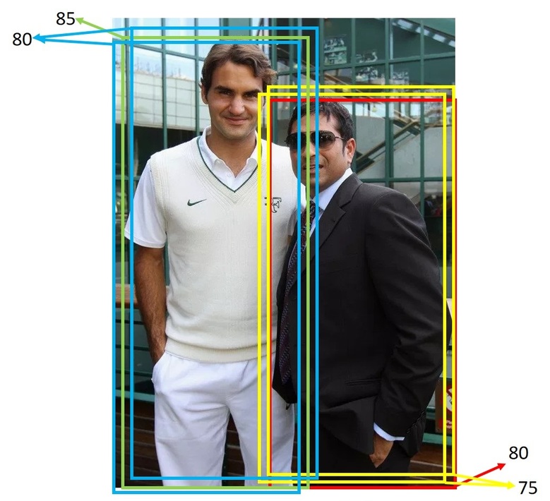
So, if you pick, say the Green box and eliminate all the overlapping boxes, you will end up eliminating boxes even for Sachin. That way, you will miss detecting Sachin.
So instead, the sane thing to do is to only eliminate boxes that have a significant overlap with the selected box.
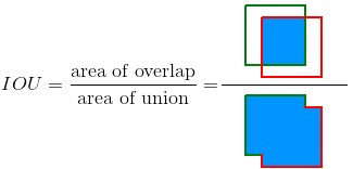
But, mathematically, how do you measure the amount of overlap? For this, we have a measure called Intersection over Union (IoU).
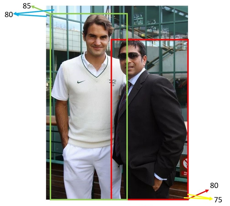
Option 2: With this, we modify the technique slightly as:
- Select the sliding window location with the highest confidence score.
- And then remove all the boxes that overlap it with an IoU > 70%.
This technique is called Non Max Suppression (NMS). This will be the result after applying NMS.
See detailed discussion on NMS here
Summary
Pre and Post processing
In general, we use:
- Sliding Windows to identify objects at different Locations
- Image Pyramid to identify objects of different sizes
These 2 techniques are applied at the input side.
At the output side, we will have multiple detections per object and some invalid detections mostly on the background regions of the image with very low confidence scores.
- So, we first do a confidence score thresholding to eliminate detections on background regions of the image.
- Then we apply NMS to get the one best detection for each of the objects in the image.
These are the 2 techniques used at the output side.
Learning
This completes the discussion on one of the first Object Detection Networks, Overfeat. You not only learnt about the network design, you also learnt many concepts, that are generic to CNNs like:
- Receptive Field
- Implementing FC layers as convolution operation
- ConvNet’s Sliding Window Efficiency
- 1x1 Convolution
- Spatial Output
- Effective Stride
- Confidence score thresholding
- Non Max Suppression and IoU
These concepts are pretty generic and you will come across them in many other papers.
In the next part (probably next week or so), we will learn about RCNN.
In the meantime, you can watch this.